Slurry Pipeline Calculations – Which Correlation Should You Use?

One of the most common questions asked by engineers who are new to slurry pipeline design is simply: “Which calculation method should I use?”

Before selecting a correlation, the engineer must first determine what they are actually trying to calculate. For example, depending upon the slurry type and the specific application, the required calculation may relate to:

the minimum velocity needed to avoid the formation of an unacceptable stationary deposit;
the hydraulic gradient or head loss at the proposed operating velocity;
the transition between laminar and turbulent flow; or
some combination of these.

The real challenge is determining which calculation methods are most appropriate for the slurry, particle-size distribution, rheology and operating conditions being considered.

Several well-known methods may appear relevant to the same project, yet each may have been developed from different test materials, pipe diameters, concentration ranges and flow regimes. The engineering challenge is therefore not simply to select a recognised correlation, but to understand the basis on which it was developed and the limits within which it can reasonably be applied.

The key message is therefore simple:

Do not begin by selecting a correlation. Begin by understanding the slurry and deciding what needs to be calculated.

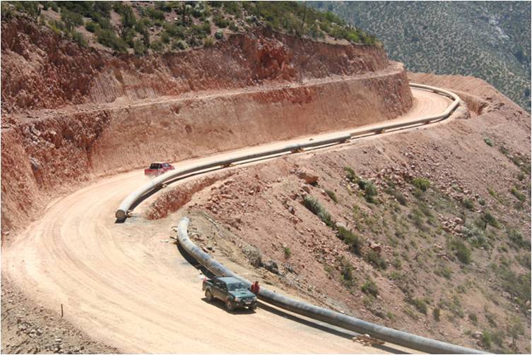
Figure 1 Slurry pipeline during construction. Long-distance slurry pipelines transport a wide variety of mineral concentrates and tailings over distances ranging from a few kilometres to several hundred kilometres. Choosing an appropriate hydraulic correlation is a critical component of successful pipeline design.

Not all slurries behave in the same way

The word slurry covers an extremely broad range of mixtures. Examples include:

coarse mineral-processing slurries;
cyclone underflow;
coal slurry;
iron ore or copper concentrate;
conventional tailings;
thickened tailings;
red mud;
fly ash;
paste backfill; and
dredged sediments.

Although all of these contain solids suspended in a liquid, their hydraulic behaviour can be very different. No experienced slurry engineer would expect a coarse cyclone underflow, a thickened tailings slurry and a paste backfill to behave in the same way. Yet all three are commonly referred to simply as “slurry”.

A coarse mineral slurry may contain particles that settle rapidly and become concentrated near the invert of a horizontal pipe. A finely ground concentrate may behave much more uniformly across the pipe cross-section. A thickened tailings slurry may possess measurable yield stress and exhibit non-Newtonian behaviour.

Some slurries may also contain both coarse particles and a substantial fines fraction. The water and fine particles may then behave as a pseudo-carrier fluid in which the coarser particles are transported.

For this reason, broad labels such as settling and non-settling are useful only as a starting point. Good slurry pipeline design requires an understanding of:

particle size distribution;
particle density and shape;
solids concentration;
carrier-fluid properties;
fines content;
slurry rheology;
pipe diameter and roughness;
proposed velocity range; and
expected operating conditions.

Only after these have been considered should the engineer begin selecting calculation methods.

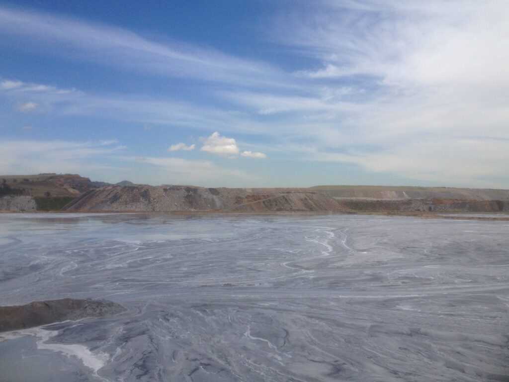
Figure 2 Fly ash TSF. Fly ash, mineral concentrates, conventional tailings and paste slurries may all behave differently in pipelines. Slurry characterisation should therefore precede correlation selection.

What Is the Minimum Acceptable Operating Velocity?

For a conventional settling slurry, one of the most important design questions is whether the selected operating velocity is sufficient to prevent the formation of an unacceptable stationary deposit. This lower operating boundary is often described using terms such as:

Deposit Velocity;
Limiting Settling Velocity;
Limit of Stationary Deposition Velocity
Critical Deposition Velocity;
Minimum Transport Velocity; or
Minimum Safe Operating Velocity.

These expressions are sometimes used interchangeably, although their precise definitions may vary between researchers and design organisations. The engineer should therefore understand how the selected method defines its calculated velocity.

This is more than simply a difference in terminology. Some methods describe the onset of stationary deposition, while others define a limiting settling condition. Although closely related, these concepts are not necessarily identical.

Deposit Velocity Is Not Necessarily at the Laminar–Turbulent Transition

A common source of confusion is the assumption that solids begin depositing because the carrier flow has become laminar. This is not necessarily the case.

A heterogeneous slurry containing settling particles may begin developing a stationary or near-stationary bed while the carrier flow remains turbulent. Deposit velocity is therefore not automatically equivalent to the velocity at which the flow changes from turbulent to laminar.

For coarse settling slurries, the relevant design question is generally whether turbulence and particle interactions are sufficient to keep the solids moving through the pipeline without forming an unacceptable stationary deposit.

For a homogeneous non-Newtonian slurry, the relevant lower operating boundary may instead relate to the transition from turbulent to laminar flow, particularly where the hydraulic gradient changes significantly across the transitional region.

These are different physical problems and generally require different calculation methods.

Common Deposit-Velocity Methods

Several methods have been developed to estimate deposit velocity for settling slurries. Among those commonly encountered are Durand-type relationships, the Wilson Nomograph, Wilson and Judge, and the later modification of Wilson and Judge (by Alan Thomas). Each method has its own origins, assumptions and range of application.

Durand-Type Deposit-Velocity Relationships

Durand-based relationships are among the best-known methods in slurry pipeline engineering. They are historically important and remain useful for illustrating the influence of:

pipe diameter;
particle size;
relative solids density;
solids concentration; and
carrier-fluid properties.

Wilson Nomograph

The Wilson Nomograph provides a practical method for estimating the deposit velocity of coarse, freely settling particles. It is particularly useful when dealing with true coarse-particle transport in a relatively low-viscosity carrier fluid. Its graphical format also makes it a valuable teaching tool because it demonstrates the influence of particle settling behaviour, pipe diameter and solids concentration. However, it should not be expected to represent all mineral slurries.

Where the slurry contains a substantial fines fraction, the viscosity and density of the effective carrier fluid may differ considerably from those of water. A method developed for coarse solids transported in water may then become inappropriate unless those effects are properly considered.

Wilson and Judge

Wilson and Judge remains one of the most widely used methods for estimating deposit velocity in heterogeneous mineral slurries. Its popularity stems from the fact that it provides practical engineering calculations while still reflecting the important influence of particle size, pipe diameter and slurry characteristics. Like all empirical methods, however, it should be applied within the range of conditions for which it was developed.

Modified Wilson and Judge — Alan Thomas

Many modern mineral slurries contain sufficient fines for the mixture of water and fines to behave as a pseudo-carrier fluid transporting the coarser particles. Alan Thomas modified the Wilson and Judge approach to better account for this behaviour, making it particularly applicable to many modern concentrate and tailings pipelines where the fines fraction has a significant influence on transport behaviour.

Allowing a Margin Above the Calculated Deposit Velocity

The calculated deposit velocity should rarely become the operating setpoint without further consideration. A practical operating velocity should usually include an appropriate margin to allow for uncertainty in:

slurry characterisation;
particle size distribution;
solids concentration;
pipe internal diameter;
pipe roughness;
pump performance;
instrument accuracy;
changing production conditions; and
the correlation itself.

The appropriate margin is project-specific. Operating too close to the calculated deposit velocity may increase the risk of bed formation during routine variations in throughput or solids concentration. Conversely, selecting an unnecessarily high velocity can increase:

friction losses;
pumping power;
wear;
particle degradation; and
whole-of-life cost.

The objective is therefore not simply to operate as fast as possible. It is to establish a reliable operating window. If in doubt, a typical recommended margin is the greater of 10% or 0.3 m/s above the calculated deposit velocity.

What Hydraulic Gradient Will Occur?

Once an acceptable operating velocity range has been established, the engineer must calculate the hydraulic gradient or head loss. For a water pipeline, friction loss can generally be calculated using an accepted single-phase method such as Darcy–Weisbach. For a slurry pipeline, the calculation may need to account for:

carrier-fluid friction;
additional energy required to support and transport solids;
concentration gradients across the pipe;
particle settling velocity;
sliding or moving beds;
pseudo-carrier-fluid behaviour;
slurry rheology; and
the interaction between coarse and fine particle fractions.

Different methods represent these effects in different ways.

Common Heterogeneous Head-Loss Methods

Durand/Condolios-Type Methods

Durand and Condolios-type methods are historically important approaches for estimating the additional hydraulic gradient associated with heterogeneous slurry transport. They often express slurry head loss in relation to the hydraulic gradient of the carrier fluid, together with an empirical excess-gradient relationship.

These methods are comparatively straightforward and remain useful for preliminary calculations and sensitivity studies. However, their simplicity should not be confused with universal applicability. Their calculation depend upon the empirical factors used and the degree to which the design slurry resembles the experimental data from which the method was developed.

Wasp Method

The Wasp method is closely associated with the hydraulic transport of coal slurry and broadly graded solids. One of its important features is the treatment of different particle-size fractions according to whether they behave more homogeneously or heterogeneously. This makes it conceptually useful for slurries with broad particle size distributions.

However, its origins should not be ignored. Although the Wasp method has been applied beyond coal, successful use in one industry does not prove universal applicability to all mineral slurries. The engineer should consider whether differences in particle density, shape, grading and carrier-fluid behaviour are significant for the proposed application.

SRC Two-Layer Model

The SRC two-layer model (which is a proprietary method) represents the slurry as two interacting regions:

a more concentrated lower layer; and
an upper region containing a more dilute suspension.

This provides a more physical representation of stratified slurry transport than simpler excess-gradient correlations. The model may be particularly useful where there is a substantial concentration gradient or a moving bed near the pipe invert.

Its additional sophistication, however, requires more input data and does not remove the need for engineering judgement. A more complicated model is not automatically more accurate if its inputs are poorly characterised.

Wilson-Based Head-Loss Methods

A number of methods associated with Wilson and his co-researchers (e.g. Thomas) have also been developed for calculating heterogeneous slurry hydraulic gradients. These should not be confused with:

the Wilson Nomograph; or
the Wilson and Judge deposit-velocity method.

Where a Wilson-based method is used, the exact method should be identified rather than referring generically to a Wilson correlation. This is important because the same researcher’s name may be associated with methods calculating different aspects of slurry behaviour.

When the Fines Become the Carrier Fluid

Many mineral slurries cannot be represented adequately as coarse particles transported in clean water. Where the slurry contains a sufficiently large concentration of very fine particles, the mixture of water and fines may behave as a pseudo-carrier fluid. The coarser particles are then transported within this modified vehicle rather than directly in water. The pseudo-carrier fluid may have:

a higher density than water;
a higher apparent viscosity;
non-Newtonian rheological properties; or
some combination of these.

This can materially affect both deposit velocity and head loss. The difficulty is that there is no single fines concentration at which the slurry suddenly changes from a water-carrier system to a pseudo-carrier-fluid system. The transition depends upon:

particle size distribution;
fines mineralogy and shape;
solids concentration;
interparticle forces;
carrier-fluid chemistry; and
applied shear rate.

Laboratory particle-size and rheological data therefore become particularly important.

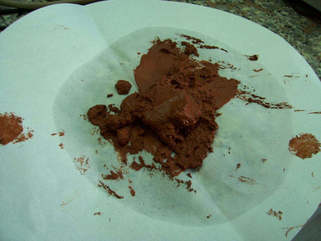
Figure 3 Red mud at 55% solids c/w. High-fines tailings may exhibit pseudo-homogeneous flow behaviour, requiring different modelling approaches to conventional coarse settling slurries.

Why Calculation Accuracy Matters More for Long Pipelines

A small difference in the calculated hydraulic gradient may be relatively unimportant for a short processing-plant pipeline but become highly significant when accumulated over a long-distance pipeline.

Consider two technically plausible methods that calculate hydraulic gradients of 3.5 metres per 100 metres and 4.0 metres per 100 metres.

The difference is only 0.5 metres of head loss per 100 metres of pipeline.

For a pipeline that is 250 metres long, the difference in calculated friction head is 1.25 metres.
For a pipeline that is 40 kilometres long, the difference becomes 200 metres.

The correlations have not diverged more on a percentage basis. The same difference in calculated hydraulic gradient has simply accumulated over a much longer distance.

A difference of this magnitude may completely change the economics of a project by influencing:

pump selection;
the number and spacing of pump stations;
pipeline pressure class;
motor power;
electrical infrastructure;
energy consumption;
operating cost; and
project viability.

This is why an approximate correlation may be adequate for a preliminary assessment of a short plant pipeline but unacceptable as the sole basis for designing a long-distance slurry transport system.

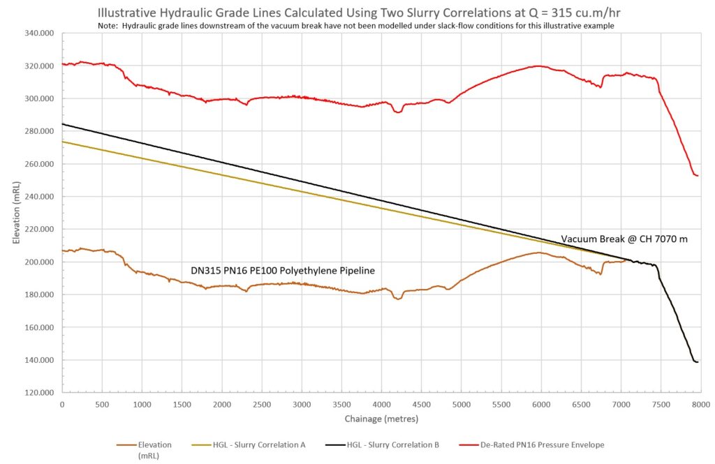
Figure 4 Illustrative hydraulic grade lines calculated using two alternative slurry correlations for the same flow rate and pipeline. Both calculations are referenced to atmospheric pressure at the vacuum break at CH 7070 m. The difference in calculated hydraulic gradient therefore accumulates upstream, resulting in materially different pump discharge heads. The hydraulic grade lines downstream of the vacuum break have not been modelled under slack-flow conditions.

Is the Flow Laminar or Turbulent?

For homogeneous and pseudo-homogeneous slurries, head-loss calculation commonly requires the slurry rheology to be characterised. Rheological models frequently used include:

Bingham Plastic;
Power Law; and
Herschel–Bulkley.

These models describe different relationships between shear stress and shear rate.

Selecting a rheological model simply because it is available in software is rarely sufficient. It should be supported by laboratory rheological testing over a shear-rate range relevant to the pipeline.

Transition Matters

The transition between laminar and turbulent flow is important because the mechanism governing head loss changes across the transition region. A method that calculates laminar flow accurately may not adequately calculate turbulent flow. Similarly, a turbulent friction-factor correlation should not be extended into the laminar region without justification.

This distinction becomes particularly important for long-distance pipelines where relatively small errors in hydraulic-gradient calculation accumulate over many kilometres.

Research on non-Newtonian slurry transport treats the identification of transition and the calculation of turbulent friction as important and distinct hydraulic problems.

Common Rheology-Based Methods

Once the slurry has been characterised as a homogeneous or pseudo-homogeneous non-Newtonian fluid, several well-established calculation methods are available for determining flow regime and hydraulic gradient. The following are among the methods most commonly encountered in practice.

Darby–Melson: For calculating the head loss for Bingham Plastic slurries across different flow regimes.

Dodge–Metzner: For calculating the head loss for the turbulent flow of power-law fluids.

Irvine Methods: For calculating the head loss for power-law and generalised non-Newtonian slurries.

Slatter Methods: Specifically address transition and turbulent flow of non-Newtonian slurries. They are particularly relevant where pipe roughness, yield stress and non-Newtonian turbulent behaviour need to be considered explicitly.

Wilson-Thomas: For calculating the head loss for the turbulent flow of non-Newtonian slurries.

Thomas-Wilson: For calculating the transition velocity of Bingham Plastic slurries.

The following table is intended as a practical starting point rather than an exhaustive literature review. Some methods calculate deposit velocity, some calculate hydraulic gradient or friction factor, and others identify the transition between laminar and turbulent flow. Several methods may therefore be required for a single pipeline assessment. KASA Redberg’s Advanced Slurry Pumping & Piping training manual contains additional details for these methods including worked example problems.

Common Slurry Pipeline Calculation Methods

The following table summarises some of the more commonly encountered slurry pipeline calculation methods. It is intended as a practical guide only and should not be regarded as an exhaustive review of the published literature.

Method	Primary Calculation	Most Appropriate For	Comments
Minimum Transport / Deposit Velocity Calculations
Durand-type Deposit Velocity	Limiting Settling Velocity	Conventional heterogeneous settling slurries	Historic empirical method for estimating minimum transport velocity.
Wilson Nomograph	Limit of Stationary Deposition	True coarse-particle settling slurries	Practical graphical method for coarse particles transported in a low-viscosity carrier fluid. Less applicable where significant fines modify the effective carrier fluid.
Wilson & Judge	Deposit Velocity	General heterogeneous mineral slurries	Widely used practical method for settling particles transported in turbulent flow. Applicable within the limits of the original experimental data.
Modified Wilson & Judge (Thomas)	Deposit velocity	Widely graded mineral slurries containing sufficient fines to form a pseudo-carrier fluid transporting the coarser particles	Extends the Wilson & Judge approach by recognising the influence of the pseudo-carrier fluid on the transport of the coarser fraction. Particularly applicable to many modern tailings and concentrate pipelines where fines significantly influence slurry behaviour.
Hydraulic Gradient (Head Loss) Calculations
Durand / Condolios	Hydraulic gradient (head loss)	Conventional heterogeneous settling slurries	Classical excess-gradient approach. Simple and widely recognised, but empirical and dependent upon appropriate selection of the empirical coefficients.
Wasp	Hydraulic gradient (head loss)	Broadly graded slurries (originally coal)	Accounts for different particle size fractions behaving differently within the flow. Frequently applied outside coal, but users should understand its origins.
SRC Two-Layer Model	Hydraulic gradient (head loss)	Stratified or two-layer heterogeneous flow	Represents the slurry as interacting upper and lower layers. Requires more detailed slurry characterisation than simpler empirical methods.
Wilson Heterogeneous Slurry Methods	Hydraulic gradient (head loss)	Coarse and graded mineral slurries	Wilson developed several heterogeneous slurry head-loss methods. These should not be confused with the Wilson Nomograph, Wilson & Judge deposit velocity methods or the Wilson–Thomas non-Newtonian methods.
Wilson-Thomas	Turbulent hydraulic gradient	Homogeneous and pseudo-homogeneous Bingham plastic slurries	Calculates turbulent friction losses for non-Newtonian slurries. Used together with a laminar-flow method and an appropriate transition criterion.
Buckingham-Reiner	Laminar hydraulic gradient	Bingham plastic slurries	Classical laminar-flow solution for Bingham plastics. Not applicable for turbulent flow.
WASC	Hydraulic gradient	Heterogeneous and broadly graded mineral slurries	Modern family of methods developed by Wilson, Addie, Sellgren and Clift, widely used in slurry pipeline engineering. Includes approaches applicable to several slurry transport regimes and is documented extensively in Slurry Transport Using Centrifugal Pumps.
Darby–Melson	Hydraulic gradient	Bingham plastic slurries	Practical engineering method covering laminar, transitional and turbulent flow. Requires reliable rheological data.
Dodge–Metzner	Turbulent hydraulic gradient	Power-law fluids	Turbulent friction-factor method used once the flow has been established as turbulent. Normally used in conjunction with the Metzner–Reed generalised Reynolds number.
Irvine	Hydraulic gradient	Power-law fluids	Alternative turbulent-flow calculation used for some non-Newtonian fluids. Users should confirm the specific formulation being implemented.
Darby	Hydraulic gradient	General non-Newtonian fluids	General friction-factor relationships applicable to several rheological models. The exact Darby formulation should be identified.
Slatter	Turbulent hydraulic gradient	Yield-stress and other non-Newtonian slurries	Advanced methods developed for non-Newtonian slurry transport, particularly where pipe roughness and yield stress significantly influence turbulent flow.
Flow Regime Identification
Thomas-Wilson	Laminar–turbulent transition velocity	Bingham plastic slurries	Used to determine whether laminar or turbulent flow calculations are appropriate.
Metzner–Reed	Laminar–turbulent transition velocity	Power-law and other time-independent non-Newtonian fluids	Widely accepted framework for identifying the flow regime prior to selecting an appropriate friction-factor relationship. Forms the basis of many subsequent non-Newtonian pipe-flow methods.

Understand Where the Correlation Came From

Unlike the Darcy–Weisbach equation, most slurry calculation methods contain empirical relationships derived from laboratory testing, field measurements or both. They are developed from combinations of:

theoretical hydraulic principles;
dimensional analysis;
laboratory pipe-loop testing;
field measurements; and
empirical curve fitting.

Researchers naturally attempt to relate slurry behaviour back to first principles. However, slurry transport is influenced by complex interactions involving:

turbulence;
gravity;
particle settling;
particle collisions;
concentration gradients;
fluid rheology;
pipe-wall interactions; and
particle size and shape.

Empirical factors are therefore almost unavoidable. This does not make a correlation invalid. It means that the engineer should understand the experimental data from which it was developed. Questions worth asking include:

What solids and solids concentrations were tested?
What was the particle size distribution?
What was the particle density and shape?
What pipe diameters were used?
Was the carrier fluid water or a fines-based vehicle?
Were the tests conducted in laboratory loops or operating pipelines?
Was the method developed to calculate deposit velocity, hydraulic gradient or transition?
Is the proposed application within or outside the original data range?

A correlation will generally have the greatest credibility when applied to a slurry and operating range reasonably similar to those used during its development.

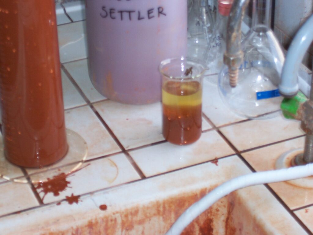
Figure 5 Slurry laboratory. Slurry correlations are generally developed from experimental testing supported by hydraulic theory and empirical curve fitting. Their applicability depends partly upon how closely the design slurry resembles the original test material and operating conditions.

Use Multiple Methods—But Compare Like with Like

Where two appropriate methods produce materially different results, the first response should not be to assume that one is “wrong”. Instead, revisit the slurry characterisation and the assumptions behind each method. Differences between methods often reveal as much about the slurry as they do about the correlations themselves.

Wherever practical, an important slurry pipeline should be assessed using more than one suitable method. This can provide:

An upper and lower estimate;
an indication of model uncertainty;
an opportunity to identify anomalous results; and
a basis for targeted laboratory or pilot-scale testing.

However, the comparisons must be meaningful. A deposit-velocity method should be compared with another deposit-velocity method. A heterogeneous head-loss model should be compared with another method suitable for the same slurry regime.

Suppose two suitable deposit-velocity methods calculate 2.2 m/s and 2.6 m/s. That difference requires investigation because it may materially influence the selected operating velocity. Similarly, if two appropriate hydraulic-gradient methods calculate 3.5 metres per 100 metres and 4.0 metres per 100 metres, the significance of the difference depends strongly upon pipeline length.

The purpose of sensitivity analysis is not necessarily to decide which correlation is correct. It is to understand how strongly the design depends upon the calculation method.

Laboratory Testing Remains Important

For high-value or long-distance pipelines, correlation selection should ideally be supported by representative laboratory testing. Testing may include:

particle size distribution;
solids density;
solids concentration;
settling tests;
rheological testing;
pipe-loop pressure-gradient testing;
deposition testing;
wear testing; and
restart testing following shutdown.

No laboratory programme can reproduce every future operating condition. However, representative testing can reduce reliance upon correlations developed from unrelated slurries and provide a basis for calibrating the selected model. The value of testing increases when:

the pipeline is long;
the static and friction heads are high;
several pump stations are required;
the slurry is unusual;
the available design margin is small;
the solids concentration will vary significantly; or
failure to restart the pipeline would have serious consequences.

Spreadsheet or Commercial Hydraulic Software?

Commercial hydraulic modelling software can be extremely useful. It is particularly valuable for:

complex pipe networks;
multiple pump stations;
several operating scenarios;
changing elevations;
control-valve analysis;
surge analysis;
sensitivity studies; and
rapid comparison of system configurations.

However, a well-programmed spreadsheet may be equally useful—or more useful—for analysing a single slurry pipeline. A spreadsheet allows the engineer to:

see the calculation sequence;
compare several correlations side by side;
modify assumptions transparently;
review units and intermediate values;
identify which method calculates each output; and
understand why results differ.

Commercial hydraulic software and spreadsheets are both engineering tools. Neither replaces engineering judgement. A useful analogy is the difference between a nail gun and a hammer. A nail gun can complete a full day of repetitive nailing far more efficiently than a hammer. However, it does not decide whether the correct structure is being built.

In the same way, hydraulic modelling software can perform large numbers of calculations quickly, but it cannot independently determine whether the selected correlation represents the slurry being analysed.

The presence of a correlation in a software package does not prove that it is suitable for a particular project. The engineer remains responsible for selecting the physics.

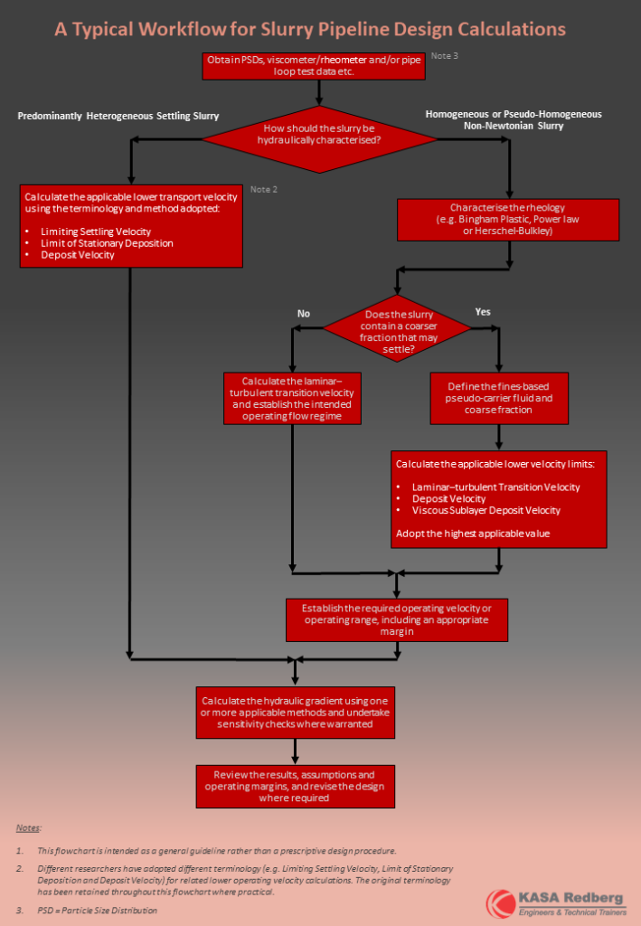
Figure 6 A typical slurry pipeline calculations workflow.

Note 1: For pseudo-homogeneous slurries containing a coarse particle fraction, the deposit velocity shown in Figure 6 will commonly be calculated using the Modified Wilson & Judge method.

Note 2: It should also be recognised, whilst not mentioned specifically in Figure 6, that laminar flow is not always undesirable. Some high-concentration tailings and paste pipelines are intentionally designed to operate in the laminar regime where the resulting pressure gradient, pumping requirements and operational considerations remain acceptable.

Final Thoughts

Successful slurry pipeline design begins not by selecting a familiar equation or software option, but by understanding the slurry itself.

Once the slurry has been properly characterised, suitable calculation methods can be selected, their assumptions understood, their results compared and engineering judgement applied.

Want to learn more?

Calculating deposit velocity and slurry head loss represents only part of successful slurry pipeline design. Reliable systems also require an understanding of:

slurry and rheological characterisation;
pump selection;
pump derating;
operating velocity limits;
pipeline wear;
solids concentration effects;
system and pump interaction;
series pumping;
hydraulic transients;
shutdown and restart; and
practical operating constraints.

These topics are explored in greater depth during KASA Redberg’s Advanced Slurry Pumping & Piping training course. The course focuses on practical engineering design and the application of sound judgement rather than simply entering data into equations or accepting software defaults. This course is presented publicly every August and can also be presented at your place of work at any other time throughout the year.